
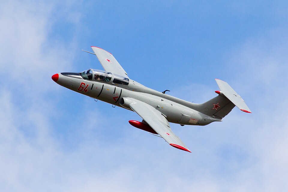
The L-29 Delfín – Dolphin (NATO reporting name ‘Maya‘) was a military jet trainer designed in the late 1950s by the Czechoslovak company Aero. It was developed to compete with Soviet and Polish designs for the standard trainer of Warsaw Pact countries. The L-29 won the competition due to its ease of handling, stability, ruggedness, and ease of maintenance.
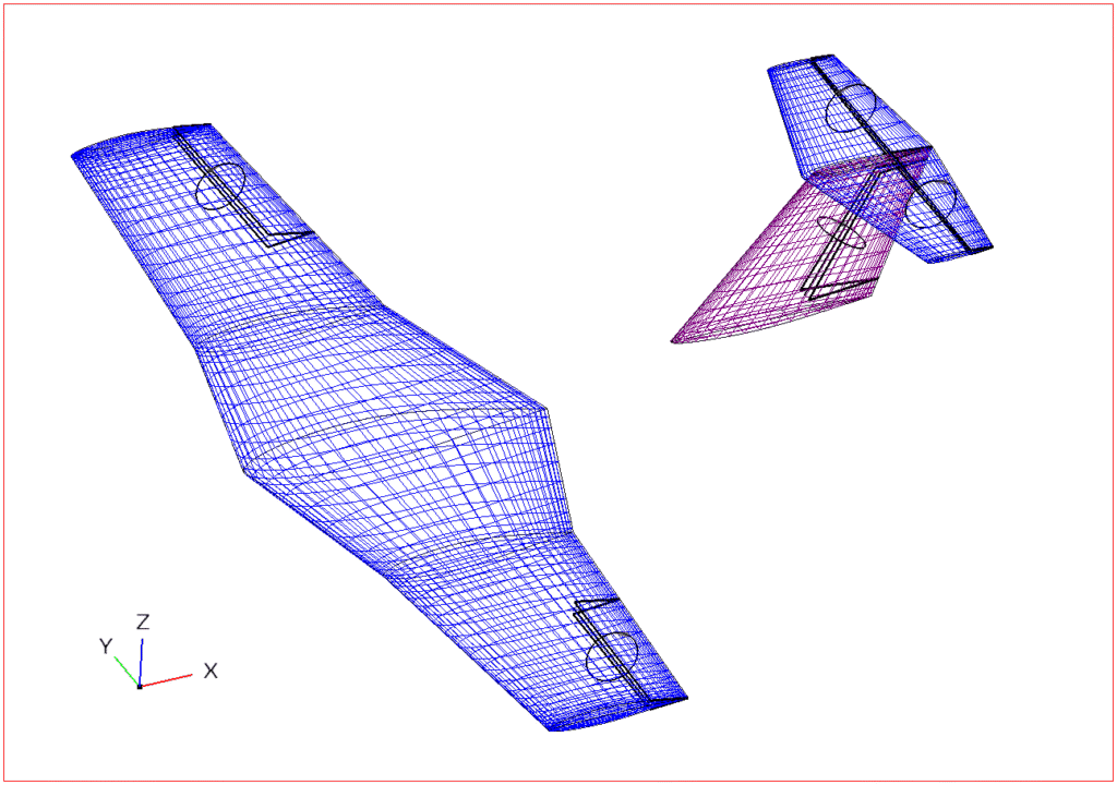
For the analysis an open source software developed by NASA OpenVSP with its solver VSPAERO was chosen. It has in-built aircraft design tool that allows for quick and simple building of a model mesh including a useful GUI. The solver is based on Vortex-Lattice Method that is not as precise as CFD with its full Navier-Stokes equations. However, it’s really computationally light-weight and – important for a hobbyist – freely available. Since the VLM models only inviscid flow, the main limitations of this approach are lack of effects of parasitic drag and no possibility of prediction of stall and its behavior.
With a great help of Kunovice Air Museum (huge thanks to Mr. Hrabec), copies of several aircraft handbooks were obtained, including Flight Manual, General Data and Operation and Maintenance manual. Having the necessary information, the model was constructed in OpenVSP editor using basic dimensions and airfoil data.
| Wingspan | 10.3 m |
| Length | 10.8 m |
| Mean aerodynamic chord | 2.04 m |
| Wing surface | 19.8 m2 |
| Airfoil at wing root | NACA 642A217 |
| Airfoil at wing parting plane | NACA 642A215 |
| Airfoil at wingtip | NACA 641A212 |
| Vertical tail airfoil | NACA 641A012 |
| Horizontal tail airfoil (data missing) | NACA 641A012 |
| Wing rigging angle | 1.5 ° |
| Outer wing dihedral | 3 ° |
The model was built including fuselage and its characteristic dorsal hump that spans all the way from the cockpit to vertical tail. In order to reach convergence of the analysis, it’s recommended to follow a few good practices:
- Use tessellation (local refinement) of mesh in places where abrupt changes of pressure field occur –at wing tips, wing to body transition, change of sweep on a part of a wing etc.
- Avoid “stripes” on a mesh – sides of mesh cells should be roughly the same length (aim for squares, avoid rectangles).
- Leave out the fuselage and analyze using only lifting surfaces. Fuselage can render the computation unstable.
- Avoid round caps on wing tips.
If the presence of the fuselage is necessary, it’s important that:
- Its shape starts and ends (longitudinally – in the direction of the air stream) with a single vertex.
- The centerline of fuselage shape is not in line with lifting surfaces. When these are aligned it leads locally to unreasonable values.
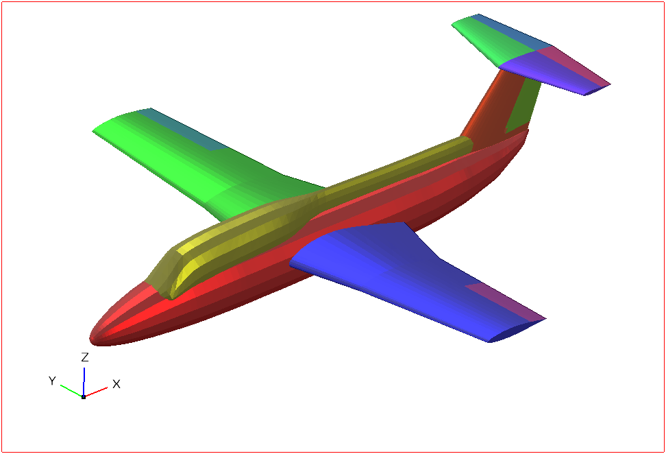
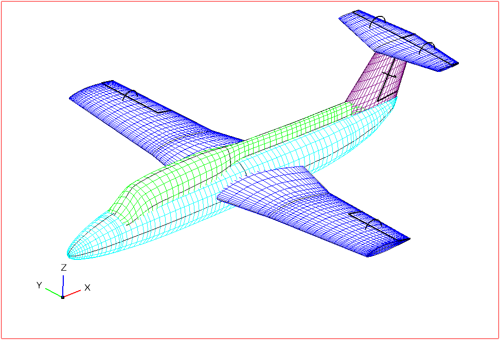
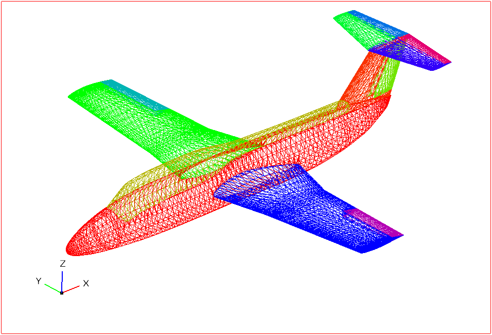
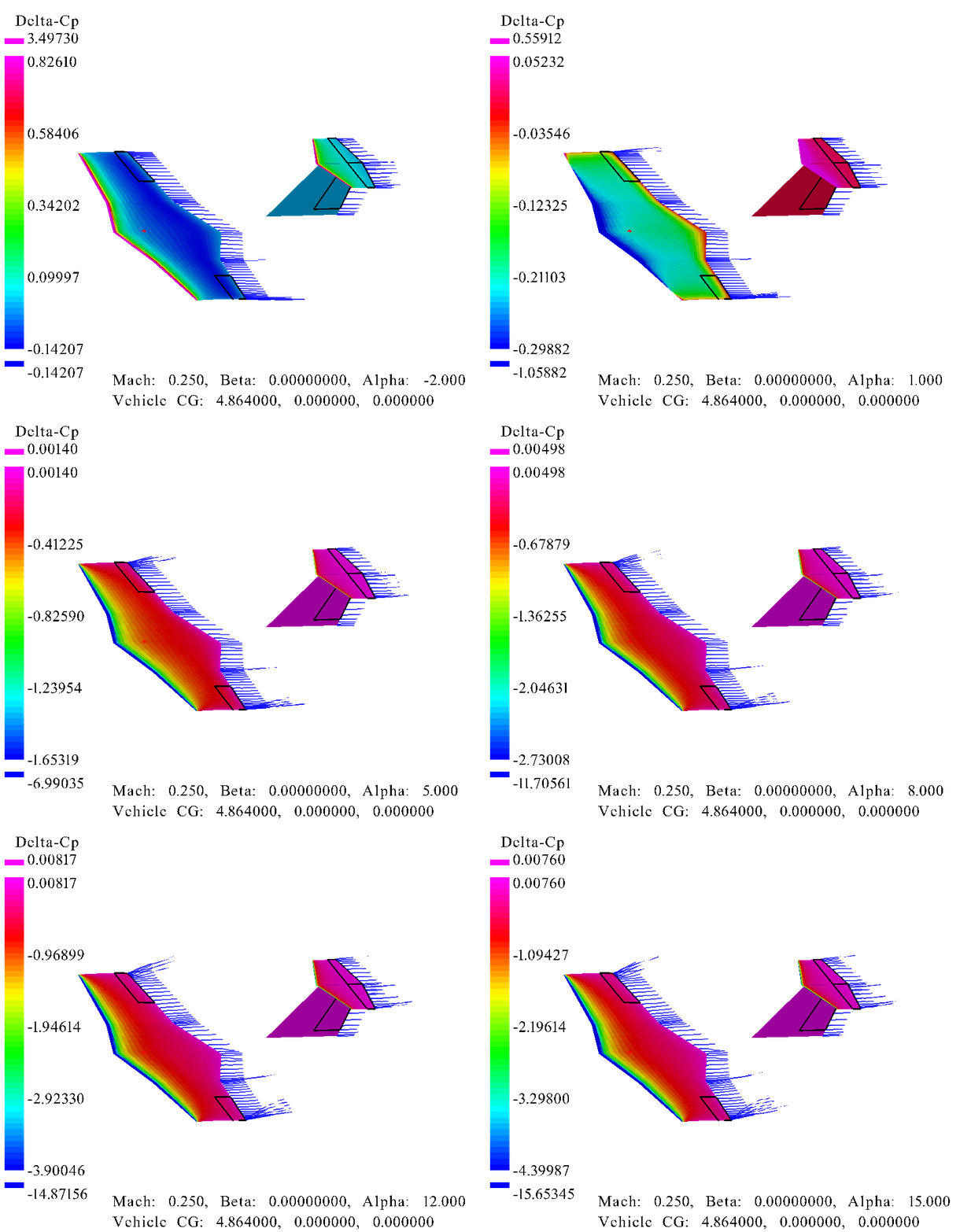
With a model built a few analyses were run in order to compare the data with references in handbooks. Lift curve and drag polar were compared. The utilized model consisted of the lifting surfaces only, as recommended. Anderson states that when using this modelling approach the error in lift coefficient is typically less than 5 %.
Alpha sweep spanning from -2 to 15 ° \(\alpha\) was performed and compared with a lift curve from the handbook. Alpha values in the handbook are related to airfoil chord line, so for each \(C_{L}\) value the wing rigging (setting) angle of 1.5 ° (relative to fuselage reference line) had to be subtracted.
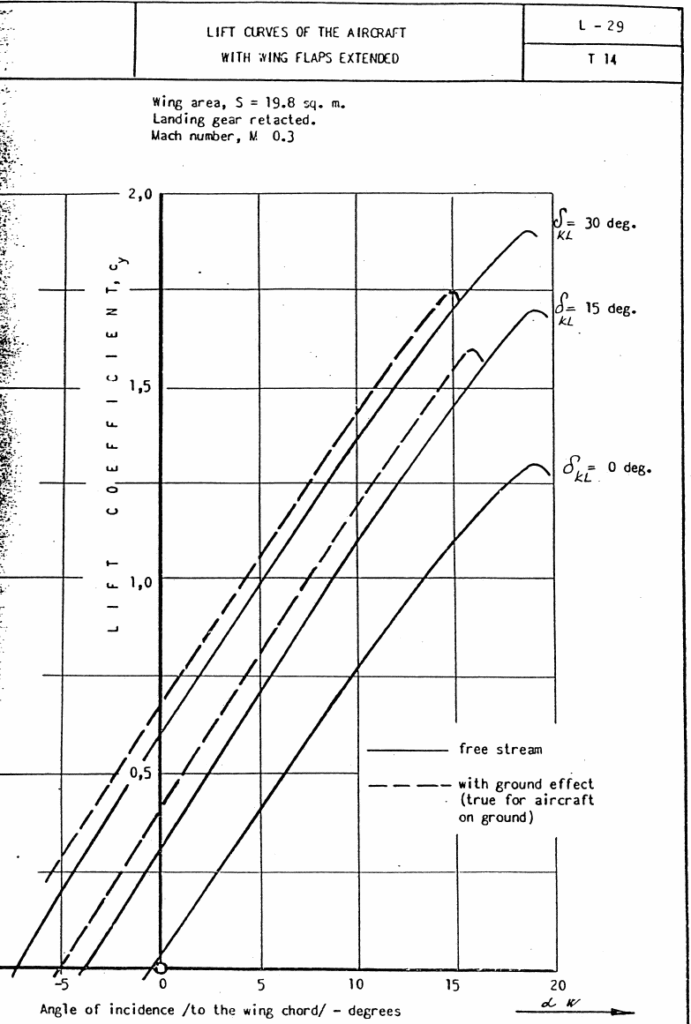
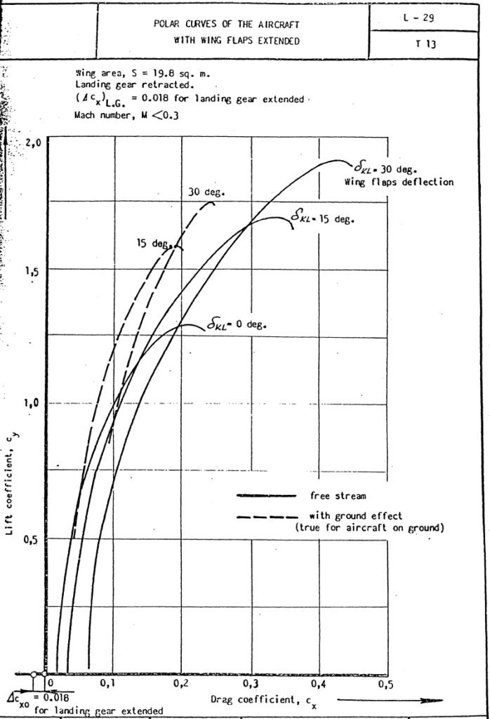
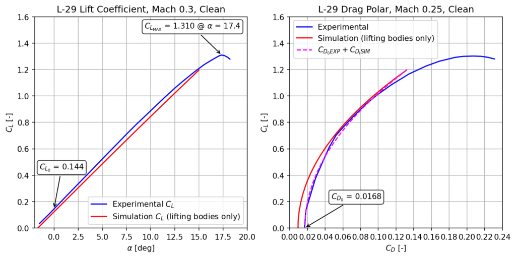
Zero-degree incidence lift coefficient value based on the handbook data equals 0.144 whereas the simulated value yields 0.122 (15.3% error). Overall, the error of simulated \(C_{L}\) values along the lift curve is smaller than 4 % \(C_{L_{\text{max}}}\). Contributing factor could be the absence of fuselage which is substituted by theoretical wing section that’s “inside” of the fuselage.
As was mentioned before, the VLM method does not simulate viscid flow, therefore no boundary layer behavior, which means that stall prediction cannot be made.
For the same reason, it cannot predict stall, the parasitic drag calculation needs to be made using other means. In case of OpenVSP, there’s an analytical tool available which offers several methods to calculate zero-lift drag (which consists of skin-friction and form drag). Default methods are Blasius and Schlichting methods. OpenVSP calculates parasitic drag first and then adds it to induced drag which it can simulate. In case of this simulation that does not include fuselage, the \(C_{D_{0}}\) value yields 0.0103. With the fuselage included we get a value of 0.01308. It’s still quite a bit lower than the handbook value of 0.0168 (22.1% error).
If we use the handbook value and sum it with the simulated induced drag (see the dashed line in the plot), the drag polar is matching nicely the experimental data up to about \(C_{L}\) of 1.0 which corresponds roughly with \(\alpha\) of 12 °.
Next post is dedicated to dynamic stability analysis of the L-29.
- Photo by Oren Rozen is licensed under CC BY-SA 3.0, via Wikimedia Commons. ↩︎
