
Given that the L-29 was highly praised for its smooth handling qualities and tame nature, we can confidently presume that the aircraft is statically stable. If it weren’t, it would likely have never completed its flight testing campaign, right? On the other hand a statically stable airframe does not necessarily have to be dynamically stable. Let’s take a closer look.
Note: in previous post we analyzed basic aerodynamic properties of the airframe using VLM method.
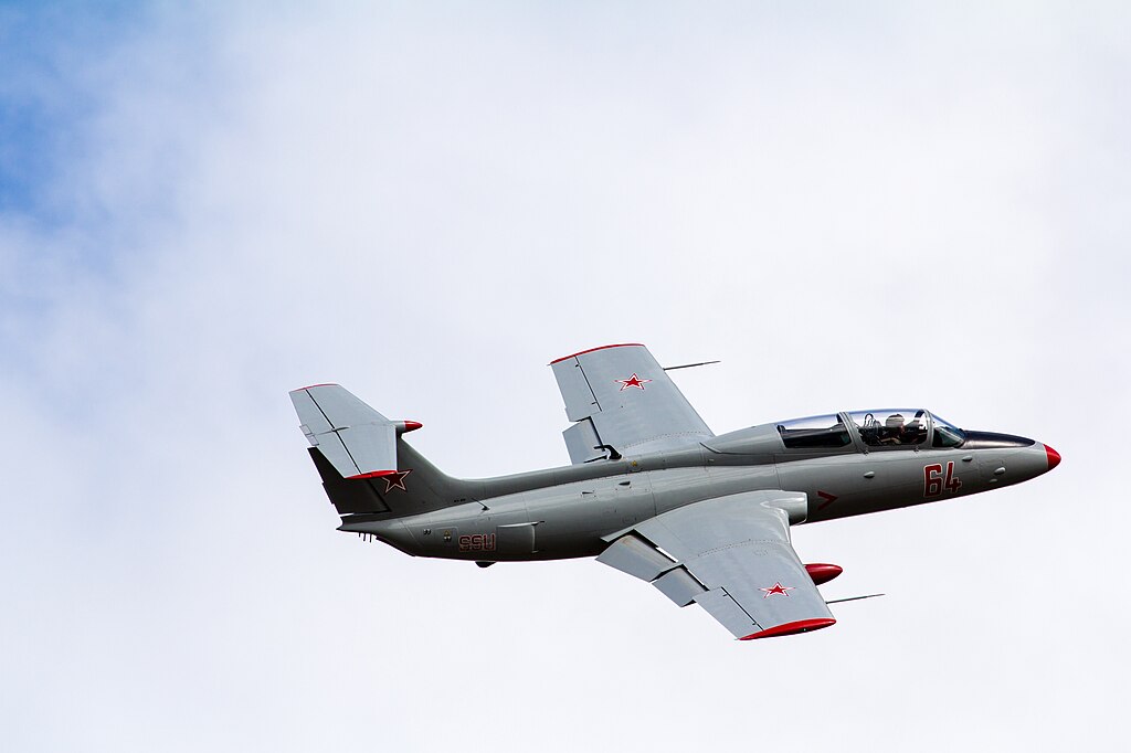
Aircraft in flight can be described by set of equations of motion. These are nonlinear, however at certain conditions – wings level, trimmed state (constant altitude) with no rotation or acceleration – the dynamics of the aircraft can be considered linear if the perturbations around this equilibrium state are small, because then the small angle approximation of trigonometric function can be utilized. When these conditions are fulfilled, we get a so called linear time-invariant system. And for these systems there are powerful tools in the control theory toolbox that can describe stability of a system.
Trimmed flight condition
Since angle of attack of a trimmed airplane differs with airspeed and altitude, let’s define a case that will be analyzed. Let’s say the L-29 is flying Mach 0.459 at altitude of 30,000 ft. It will be clear later, why this specific condition was chosen.
One analysis was run in order to get a first estimate of aerodynamic coefficients for trim analysis with these input parameters: Mach 0.459, pitch angle \(\theta\) of 0 degrees and mass of 3234 kg with CG at 23.5 % MAC which is in OpenVSP coordinate system corresponding with \(x_{B}\) = 4.884 m.
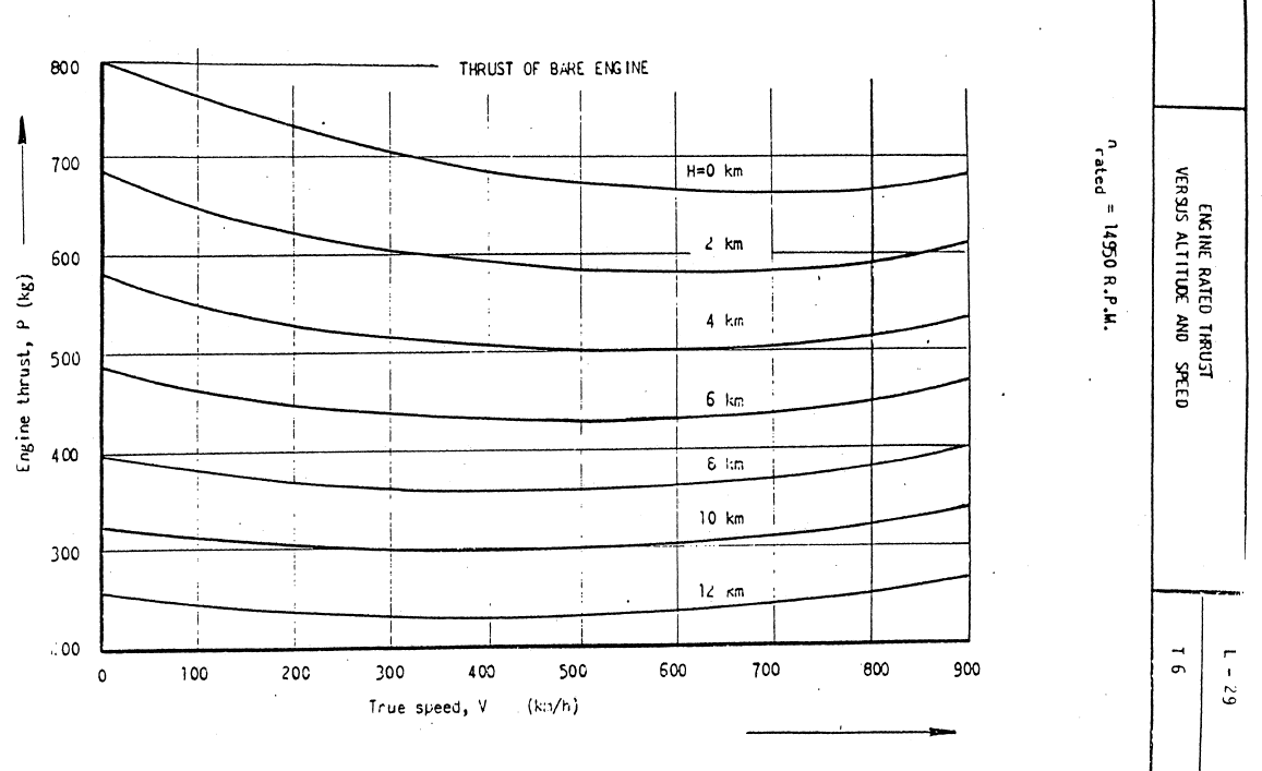
Longitudal equations of motion with a a first set of aerodynamic coefficients were fed into Newton-Raphson algorithm, a goal of which is to find a minimum value for a set of functions. That’s how our trimmed values were found after several iterations. Mach 0.459 at 30,000 ft in ISA gives true airspeed of 139.16 m/s. At this trimmed condition a pitch angle theta equals 3.2 °, elevator is deflected by -3.4 ° (negative value means trailing edge up) and required thrust is 2.12 kN. According to the handbook the M701c-500 engine of L-29 is able to produce at 9144 m and 501 km/h TAS (corresponding to given cruise condition) 320 kg of force, so around 3.1 kN at rated regime (95 % nmax), therefore achieving this trimmed state should be possible.
Stability derivatives
With the trimmed equilibrium state defined, we need to describe flight properties of the aircraft at this specific regime. OpenVSP has the ability to perform a stability analysis. The way it’s performed is simply perturbing each of the state and input variables:
- angle of attack
- sideslip angle
- roll, pitch and yaw rates
- airspeed
- elevator, aileron and rudder input
It simulates aerodynamic forces and moments with and without these perturbations and by subtracting and obtaining the differential it yields according dimensionless stability derivative coefficients. So technically, this is just a part of stability analysis. The derivatives don’t say much by themselves, at least not to my untrained eye.
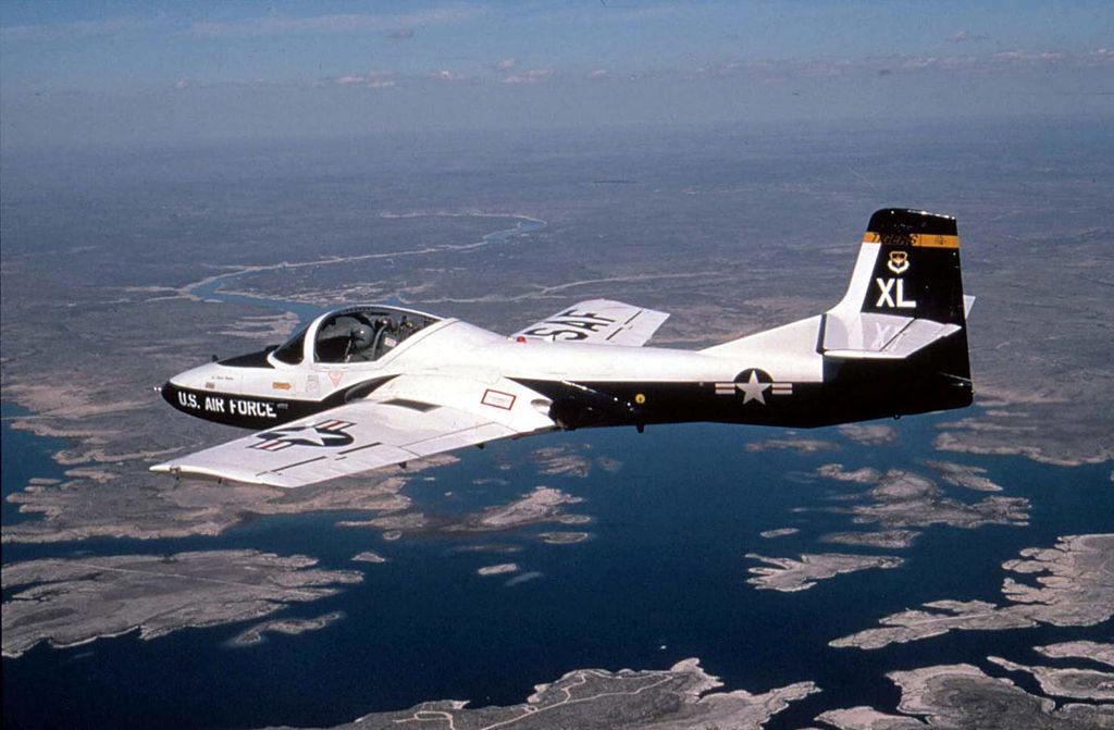
When we have our dimensionless derivatives, we’re missing the last puzzle piece – moments of inertia of the aircraft. Unfortunately, I wasn’t able to find these values anywhere. There are a few pages missing in the handbook, however I think it’s quite possible they weren’t present anyway. So in order to get a reasonable estimate I borrowed the numbers of an aircraft that is very similar in size and weight, was designed in the same era and for the same purpose. Let me introduce you to Cessna T-37 Tweet.
| Parameter | Aero L-29 | Cessna T-37 |
|---|---|---|
| Length | 10.8 m | 8.9 m |
| Wingspan | 10.3 m | 10.3 m |
| Height | 3.1 m | 2.8 m |
| Wing area | 19.8 m2 | 16.9 m2 |
| Mean aerodynamic chord | 2.04 m | 1.67 m |
| Aspect ratio | 5.36 : 1 | 6.2 : 1 |
| Airfoil | NACA 642A217 (at root) NACA 641A212 (at wingtip) | NACA 2418 (at root) NACA 2412 (at wingtip) |
| Empty weight | 2 280 kg | 1 840 kg |
| Powerplant | M701c-500 | 2x J69-T-25 |
| Maximum speed | 630 km/h | 684 km/h |
| Stall speed | 137 km/h | 137 km/h |
| Range | 870 km | 1500 km |
| Service ceiling | 10 900 m | 11 800 m |
| Rate of climb | 13.6 m/s | 17.1 m/s |
| Moment of inertia \(I_{xx}\) | N/A | 10 826 kgm2 |
| Moment of inertia \(I_{yy}\) | N/A | 4 509 kgm2 |
| Moment of inertia \(I_{zz}\) | N/A | 15 162 kgm2 |
| Moment of inertia \(I_{xz}\) | N/A | N/A |
It’s a military trainer with two seats arranged side by side and two turbojet engines. This configuration yields probably higher moment of inertia about the \(x_{B}\) (roll) axis compared with L-29, on the other hand Delfín has a bit higher dry weight, so the value hopefully won’t be too far off. About the \(y_{B}\) (pitch) axis, the values will probably differ more, given the L-29 is longer by about 2 meters. Anyway, this is the best we got.
| Parameter | Aero L-29 | Cessna T-37 |
|---|---|---|
| Weight | 3 234 kg | 2 885 kg |
| C.G. position in % MAC | 23.5 | 27 |
| Pitch angle \(\theta\) | 3.2 ° | 2 ° |
One more thing is available to our disposal: Roskam has published stability derivatives for T-37. The given values were taken at cruise regime at (you guessed it) Mach 0.459 at 30,000 ft. Now we have data for very similar aircraft to compare the L-29 with. And in order to get some frame of reference, let’s throw in a Boeing 747 in cruise condition too. The closest regime to our chosen trim state we got data for is of a jumbo jet flying at 20,000 ft, doing Mach 0.5 with pitch angle \(\theta\) of 6.8 °. The derivatives of a 747 were taken from Caughey’s course notes.
| Coefficient | Aero L-29 | Cessna T-37 | Boeing 747 |
|---|---|---|---|
| \(C_{L_{1}}\) | 0.369 | 0.378 | 0.68 |
| \(C_{D_{1}}\) | 0.0209 | 0.03 | 0.0393 |
| \(C_{L_{\alpha}}\) | 4.27 | 5.15 | 4.67 |
| \(C_{D_{\alpha}}\) | 0.297 | 0.25 | 0.366 |
| \(C_{m_{\alpha}}\) | -0.564 | -0.7 | -1.146 |
| \(C_{L_{\dot{\alpha}}}\) | N/A | 2 | 6.53 |
| \(C_{m_{\dot{\alpha}}}\) | N/A | -6.95 | -3.35 |
| \(C_{L_{q}}\) | 7.14 | 4.1 | 5.13 |
| \(C_{m_{q}}\) | -8.1 | -14.9 | -20.7 |
| \(C_{L_{M}}\) | 0.1695 | 0 | -0.0875 |
| \(C_{D_{M}}\) | 0.0113 | 0 | 0 |
| \(C_{m_{M}}\) | 0.009 | 0 | 0.121 |
| \(C_{L_{\delta e}}\) | 0.445 | 0.5 | 0.356 |
| \(C_{m_{\delta e}}\) | -1.16 | -1.12 | -1.43 |
| Coefficient | Aero L-29 | Cessna T-37 | Boeing 747 |
|---|---|---|---|
| \(C_{y_{\beta}}\) | -0.238 | -0.346 | -0.9 |
| \(C_{l_{\beta}}\) | -0.0844 | -0.0944 | -0.193 |
| \(C_{n_{\beta}}\) | 0.1089 | 0.1106 | 0.147 |
| \(C_{l_{p}}\) | -0.398 | -0.442 | -0.323 |
| \(C_{n_{p}}\) | -0.0359 | -0.0243 | -0.069 |
| \(C_{l_{r}}\) | 0.1131 | 0.0926 | 0.212 |
| \(C_{n_{r}}\) | -0.121 | -0.139 | -0.278 |
| \(C_{l_{\delta a}}\) | -0.2306 | -0.181 | -0.0129 |
| \(C_{n_{\delta a}}\) | 0.001 | 0.0254 | -0.0015 |
| \(C_{y_{\delta r}}\) | 0.1502 | 0.2 | 0.1448 |
| \(C_{l_{\delta r}}\) | 0.0235 | 0.015 | 0.0039 |
| \(C_{n_{\delta r}}\) | -0.0736 | -0.0365 | -0.1081 |
Note that the coefficients of rolling and yawing moment that were given by Roskam had opposite signs. That is caused by different notation of positive aileron deflection. For example according to Cook the positive aileron deflection is given by RH trailing edge down which produces negative rolling moment (the \(x_{B}\) axis of body coordinate system is going through the nose forward).
Linearized equations of motion
With the gap filled that was caused by missing moments of inertia, the linear dimensional equations of motion can be constructed. Linearization process with a presumption of trimmed flight condition yields two decoupled sets: one for longitudinal (pitch-related movement) and one for lateral (roll and yaw) motion of a system. In reality the motion coupling from longitudinal to lateral is negligible. That’s not the case the other way around. On the other hand, the linearization was done under the assumption of small perturbations. And as a bonus, this decoupling makes the analysis clearer and the equations easier to handle.
With the sets of equations of motion in state space form \(\dot{x} = A x + B u\), we can finally see some useful output. Let’s first check how the aircraft respond to one degree stick-fixed (constant) elevator input.
\(
A =
\begin{bmatrix}
-0.0092 & 0.0141 & 0 & -9.7914 \\
-0.1594 & -0.8393 & 137.7364 & -0.5474 \\
0.0012 & -0.1613 & -2.3511 & 0 \\
0 & 0 & 1 & 0
\end{bmatrix}, \quad
\mathbf{x} =
\begin{bmatrix}
u \\ w \\ q \\ \theta
\end{bmatrix}
\)
Above is the state matrix A and state vector representing the dynamics of L-29 in the configuration described above.
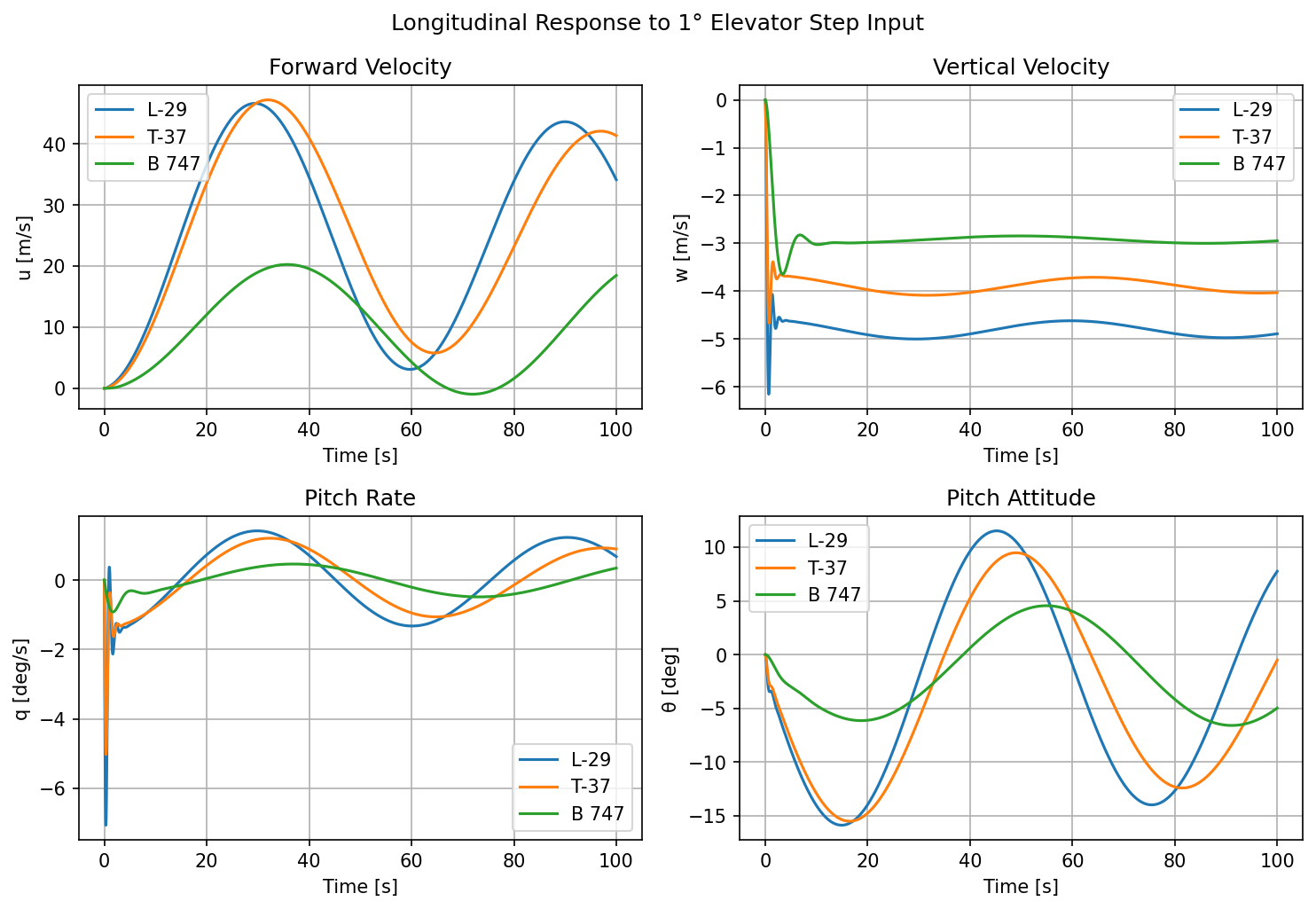
It’s apparent that the two trainers share similar properties in longitudinal response. L-29 has slightly larger elevator authority, which is most prominent in pitch rate plot – see the initial peak which shows excitation of short period mode. Even though its lift coefficient derivative due to elevator input \(C_{L_{\delta e}}\) is smaller than the one of T-37, the horizontal tail of Delfín has a longer moment arm which leads to higher pitching moment coefficient \(C_{m_{\delta e}}\). From the time domain response one can clearly see that the long period oscillation of phugoid mode of L-29 is less damped and is of lower frequency. So it can be said that behavior of T-37 is slightly nicer in this regard.
Dynamic stability modes
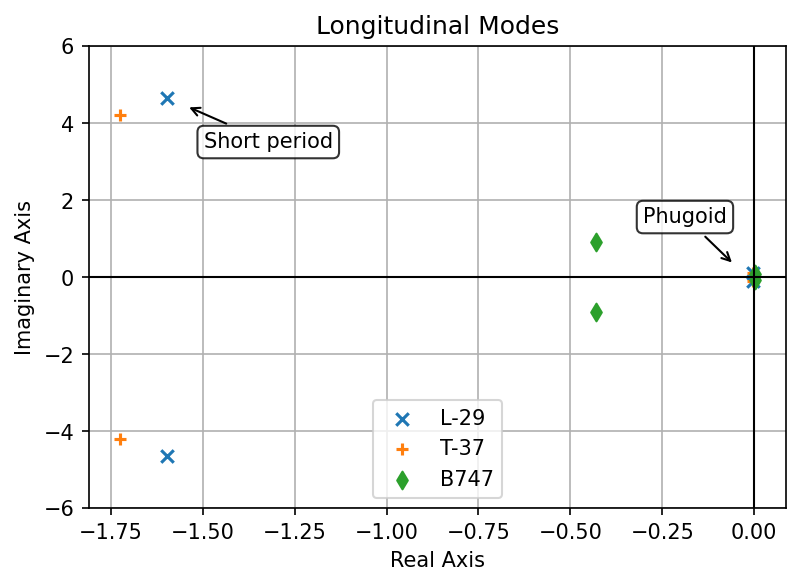
Now if we find the eigenvalues of the state matrix A, we can plot them and see how each of the two modes contributes to the longitudinal response. Note: the poles of 747 made the plot cluttered a bit but I’ve attached plots with its values at the end of this post.
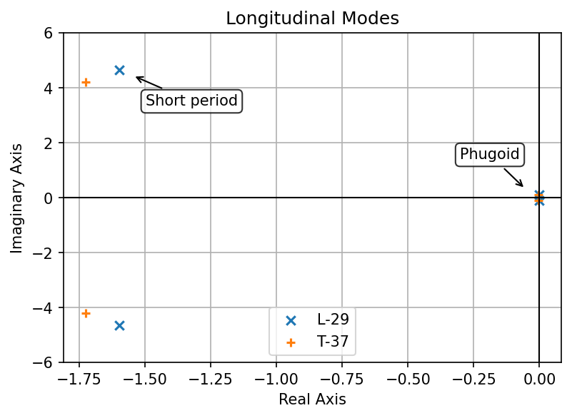
All poles in Laplace domain have negative real part for both L-29 and T-37, which means they are damped (even though just a little – damping ratio of phugoid pole of L-29 is just \(\zeta\) = 0.023). What is interesting, on the other hand, is the phugoid pole of B747 – its real part is positive, therefore unstable. However, due to very slow nature of this mode (its period is equal to \(2 \pi / \omega_{d}\) = 72.3 s) it gives more than enough time for pilot to counter it.
| Mode | Aero L-29 | Cessna T-37 | Boeing 747 |
|---|---|---|---|
| Short period | -1.5975 ± 4.6519j | -1.7238 ± 4.2041j | -0.4300 ± 0.9193j |
| Phugoid | -0.0024 ± 0.1037j | -0.0041 ± 0.0967j | 0.0011 ± 0.0868j |
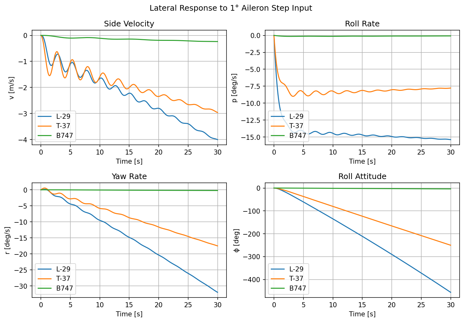
Now let’s take a look at lateral response due to aileron input. The first obvious fact is that L-29 is much more responsive in roll than T-37 (see the roll rate plot). Wingspan of both aircraft is nearly identical; the ailerons of Delfín have a bit more control surface though. This is also reflected in the rolling moment coefficient due to aileron input \(C_{l_{\delta a}}\). Let’s focus now on the roll rate plot – what could be concerning is the slope of the curve. One can note that the roll rate of T-37 after initial excitation is slowly converging back to zero. But this is not the case for L-29, this divergence is a sign of potentially unstable behavior. What is also worth mentioning is in comparison the immensely sluggish response of the 747.
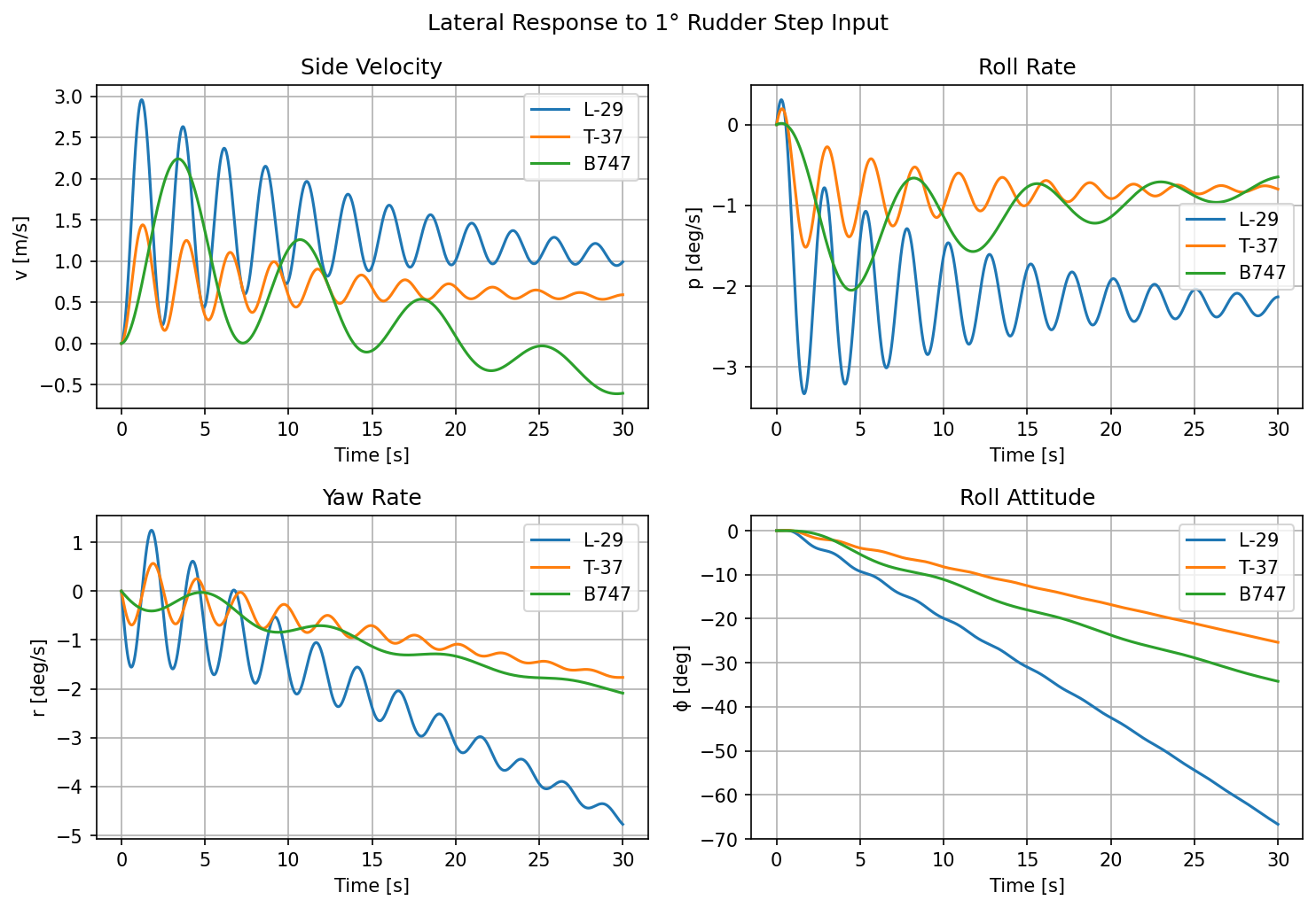
For rudder authority the similar applies that was true for elevator input. The control surface of the Tweet is slightly larger, therefore induces more side force. However, given the longer moment arm of the Delfín, its yawing moment coefficient value is in this case roughly double. Position of the rudder of the L-29 is also a bit higher above the \(x_{B}\) body (roll) axis which leads to higher rolling moment due to rudder input compared to the T-37. Both of these qualities are reflected in much larger oscillations and less damping of Dutch roll mode (coupled yaw and roll motion).
Let’s plot the poles now.
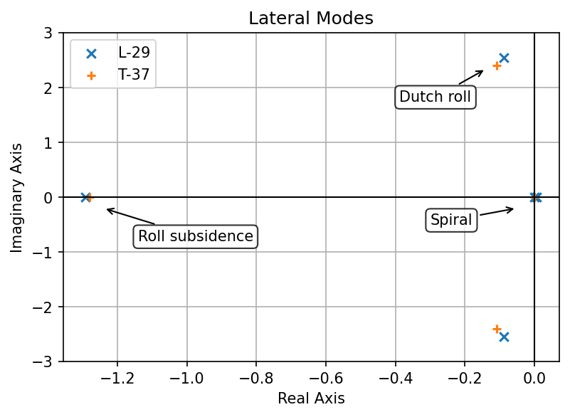
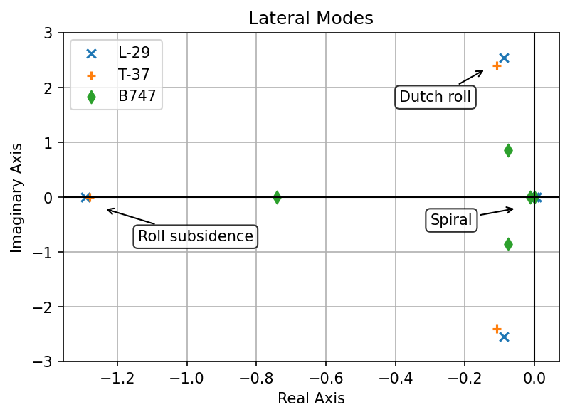
Here the poles of two aircraft are positioned relatively close to each other. However, due to scale of the plot, it’s not clear what is going on near the origin where the spiral mode resides. When we take a closer look at the actual eigenvalues we see that the real value of one of the Delfín’s poles is positive, which indicates unstable behavior.
| Mode | Aero L-29 | Cessna T-37 | Boeing 747 |
|---|---|---|---|
| Spiral | 0.0067 + 0j | -0.0014 + 0j | -0.0120 + 0j |
| Dutch roll | -0.0883 ± 2.5456j | -0.1086 ± 2.4016j | -0.0763 ± 0.8563j |
| Roll subsidence | -1.2909 + 0j | -1.2790 + 0j | -0.7408 + 0j |
| \(\psi\) dynamics | 0 + 0j | 0 + 0j | 0 + 0j |
Remember the possible red flag that was mentioned because of diverging roll rate due to aileron input? Here’s the culprit. Unstable spiral mode is characterized by constant increase in bank angle after a perturbation. Increased bank causes to sinking of the aircraft. If the pilot loses a visual reference (for example flying unintentionally into IMC conditions) he naturally tends to pull the stick to correct for lost altitude which makes things even worse. For pilots without instrument rating, this phenomenon could be deadly. This situation could occur in a stable aircraft too, of course, however with unstable aircraft, all it takes for this mode to be excited is a small perturbation like a cross wind gust. It poses no trouble when flying VFR or IFR though.
Here I want to mention great flight mechanics teaching material composed by Harry Smith which was of massive help and which I utilized extensively throughout the whole analysis.
- Photo by Oren Rozen is licensed under CC BY-SA 3.0, via Wikimedia Commons. ↩︎
- Photo by Staff Sgt. Andy Dunaway, Public domain, via Wikimedia Commons ↩︎

